User guide: ViSiAnnoT¶

ViSiAnnoT has been designed to be as easy to use as possible, while being highly configurable so that it could meet a variety of needs. In this section, we introduce its features and we illustrate them with examples in the context of clinical research on preterm newborns.

The dataset used for these examples is stored in a folder named “data” and is organized as follows:

Folder “interval”: files with interval data to plot over signals
- Pat01_2021-03-02T09-33-56_intervalA.txt
- Pat01_2021-03-02T09-33-56_intervalB.txt
Folder “signal”: files with signal data
- Pat01_2021-03-02T09-33-56_physio.h5 (contains ECG and respiration), synchronized with first video
- Pat01_2021-03-02T09-33-56_rr.txt, synchronized with first video
- Pat01_2021-03-02T09-33-56_tqrs.txt, synchronized with first video
- physio_2021-03-02T09-34-09.h5 (contains ECG, respiration, TQRS and RR), spanning the long recording
Folder “video”: video files for two cameras
- Pat01_2021-03-02T09-33-56_BW1.mp4
- Pat01_2021-03-02T09-33-56_BW2.mp4
- Pat01_2021-03-02T10-03-56_BW1.mp4
- Pat01_2021-03-02T10-03-56_BW2.mp4
- Pat01_2021-03-02T10-33-56_BW1.mp4
- Pat01_2021-03-02T10-33-56_BW2.mp4
Pat01_audio.wav

This dataset is not publicly available, but equivalent scripts are provided in this repository, along with an example dataset.

Video visualization with multiple cameras¶

ViSiAnnoT can be used as a simple video player. Supported formats are the ones that are supported by OpenCV (for instance .mp4 and .avi). It is possible to play as many videos as wanted simultaneously, provided that they are synchronized. This is useful when the user has video files of several synchronized cameras. The name of the video files must contain the beginning datetime of the video, so that the software can check if the videos are indeed synchronized (a shift of one second is authorized between the video files).

Here is an example:

from visiannot.visiannot import ViSiAnnoT

# video paths
path_video_1 = "data/video/Pat01_2021-03-02T09-33-56_BW1.mp4"
path_video_2 = "data/video/Pat01_2021-03-02T09-33-56_BW2.mp4"

# video configuration
video_dict = {}
video_dict["BW1"] = [path_video_1, '_', 1, "%Y-%m-%dT%H-%M-%S"]
video_dict["BW2"] = [path_video_2, '_', 1, "%Y-%m-%dT%H-%M-%S"]

# create ViSiAnnoT window
win_visiannot = ViSiAnnoT(video_dict, {})

From the sub-package visiannot we import the class ViSiAnnoT. We have a set of 2 synchronized videos, located in the folder data. The configuration dictionary video_dict specifies to ViSiAnnoT where to find the videos and how to get the beginning datetime in the video file name. Each item corresponds to one camera, the key is the camera ID and the value is a list/tuple of 4 elements:

Path to the video file,
Delimiter to get the beginning datetime in the video file name,
Position of the beginning datetime in the video file name, according to the delimiter,
Format of the beginning datetime in the video file name (see keyword argument fmt of convert_datetime_to_string()).

The instance of ViSiAnnoT must be stored in a variable in order to have the window displayed.

Fig. 2 shows a screenshot of the resulting window. At the bottom, there is the progress bar which gives the current temporal position with the red dot and allows to navigate in the video. We call the red dot “navigation point”. The temporal axis is expressed in absolute datetime. It is possible to navigate in the video by clicking in the progress bar and dragging the navigation point. The user can start/stop the video playback with the space key.

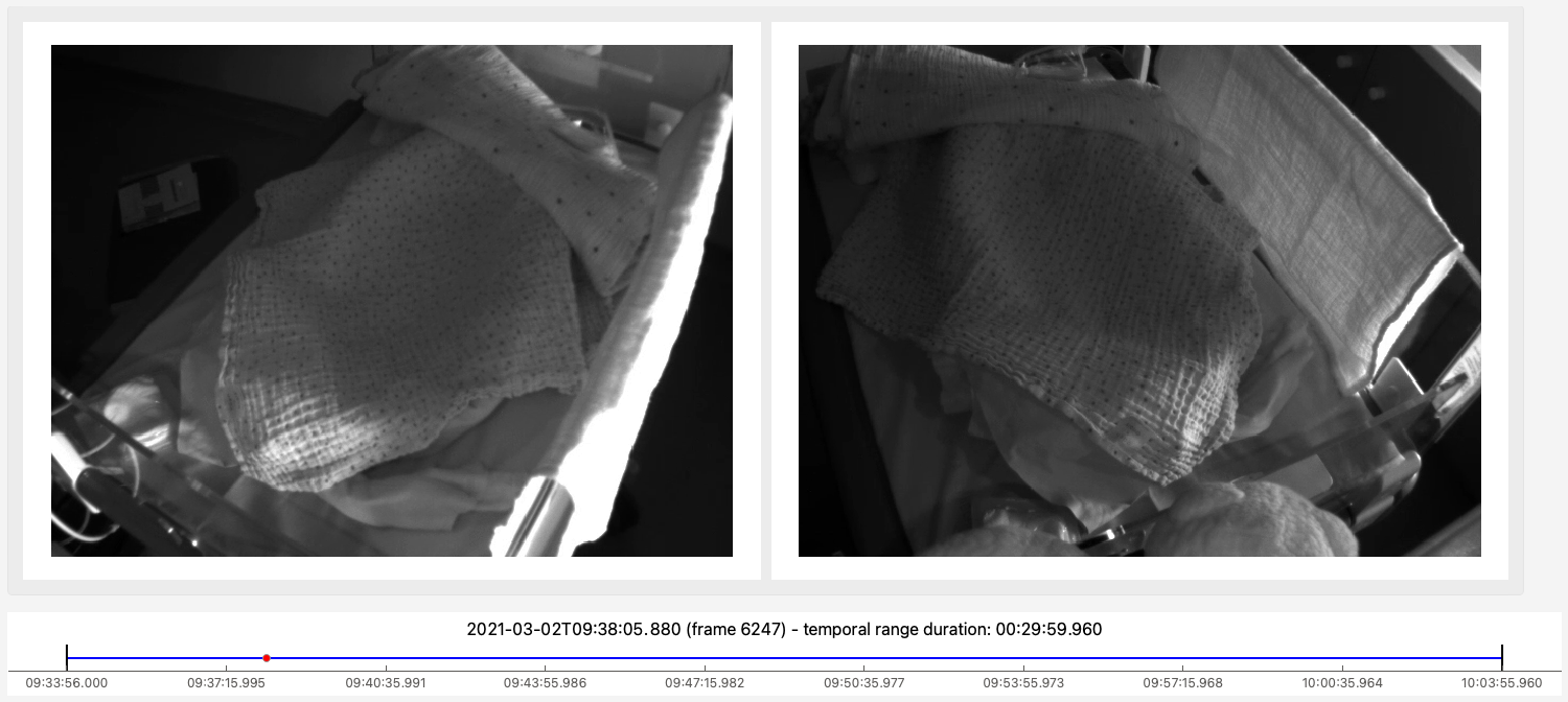
Fig. 2 Screenshot of ViSiAnnoT used as a video player¶

If audio is contained in the video file, there is currently no audio playback.

Signal visualization¶

ViSiAnnoT can be used as a simple signal viewer. The user can define as many widgets as wanted (i.e. figures) and plot as many signals as wanted in a widget. As for video visualization, the signal files should be synchronized.

Signal format¶

Supported formats are .txt, .mat, .h5 and .wav. There are two ways to store the signal:

As a vector of length $n_{sample}$ , where $n_{sample} \in \mathbb{N}$ is the number of samples in the file. In this case, the frequency is constant and must be provided by the user.
As a matrix of shape $(n_{sample},2)$ , where the first column contains the timestamp of each sample and the second column contains the value of the samples. This is particularly useful for non regularly sampled signals. The timestamps are expressed in milliseconds relatively to the beginning datetime of the file.
As a matrix of shape $(n_{sample},m+1)$ , where the first column contains the timestamp of each sample and the remaining columns contain the value of the samples of $m$ signals. This is particularly useful for several non regularly sampled signals which share the same timestamps for samples.

An example of non regularly sampled signal is the RR series, which is extracted from the physiological signal ECG (electrocardiogram). The ECG measures the electrical activity of the heart beat. During a heart beat cycle, there is a peak that can be detected. The RR series is defined as the difference between two successive peaks in the ECG. Since these peaks are not regular, the RR series is non regularly sampled.

NB: it is strongly advised to use the .h5 format instead of .txt in order to have better speed performance.

Multiple signal plots in the same widget¶

ViSiAnnoT allows to plot as many signals as wanted in the same widget. Since plotting relies on Pyqtgraph, all the configurations available in this package can be used to customize plot style (see line style and point style keyword arguments of PlotDataItem constructor).

A default plot style can be used for up to 10 signals plotted in the same widget (no symbol for points, points connected by a line). Only the color of the connecting line changes from one signal to another. Above 10 signals, it is required to manually specify the plot style.

In case several signals are plotted in the same widget, the fact that their frequencies may be different is automatically managed.

Here is an example:

from visiannot.visiannot import ViSiAnnoT

# signal paths
path_physio = "data/signal/Pat01_2021-03-02T09-33-56_physio.h5"
path_tqrs = "data/signal/Pat01_2021-03-02T09-33-56_tqrs.txt"

# define plot style
plot_style_tqrs = {
    'pen': None,
    'symbol': '+',
    'symbolPen': 'r',
    'symbolSize': 10
}

plot_style_resp = {'pen': {'color': 'm', 'width': 1}}

# signal configuration
signal_dict = {}

signal_dict["ECG"] = [
    [path_physio, '_', 1, "%Y-%m-%dT%H-%M-%S", "ecg", 500, None],
    [path_tqrs, '_', 1, "%Y-%m-%dT%H-%M-%S", "tqrs", 0, plot_style_tqrs]
]

signal_dict["Respiration"] = [
    [path_physio, '_', 1, "%Y-%m-%dT%H-%M-%S", "resp", "resp/freq", plot_style_resp]
]

# create ViSiAnnoT window
win_visiannot = ViSiAnnoT(
    {}, signal_dict, flag_pause_status=True, layout_mode=2
)

From the sub-package visiannot we import the class ViSiAnnoT. We have a set of 3 synchronized signals (ECG, respiration and QRS beat detection), located in the folder data. The configuration dictionary signal_dict specifies to ViSiAnnoT where to find the signal files, what is the frequency of the signals, how to get the beginning datetime of the signal file and how to plot. Each item corresponds to one signal widget. The key is the widget ID, which is used as Y axis label. The value is a nested configuration list where each element corresponds to one signal to plot and is a list of 7 elements:

Path to the signal file,
Delimiter to get the beginning datetime in the signal file name,
Position of the beginning datetime in the signal file name, according to the delimiter,
Format of the beginning datetime in the signal file name (see keyword argument fmt of convert_datetime_to_string()),
Key to access the data in the file (in case of .h5 or .mat, set it to '' otherwise), also used a legend - in case of 2D data with several value columns, then the column index must be specified, e.g. "key - 1" or "key - colName" if there is an attribute at key named columns with columns name being comma-separated (first column is always the timestamps),
Signal frequency (may also be a string with path to the frequency attribute in case of h5 file), set it to 0 in case of non-regularly sampled signal,
Dictionary with plot style, set to None for default plot style.

The keyword argument pause_status is set to True so that the video playback is disabled at launch. The instance of ViSiAnnoT must be stored in a variable in order to have the window displayed.

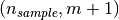
Fig. 3 shows a screenshot of the resulting window. On the first widget, there are two signals: ECG (sampled at 500 Hz) and QRS beat detection (non regularly sampled). On the second widget, there is one signal: respiration. The default plot style is used for the ECG (blue curve), whereas a custom plot style is defined for QRS beat detection (red dots) and respiration (purple curve). We call “temporal cursor” the red vertical line on the signal plots giving the current temporal position. It is linked to the red dot in the progress bar, which is above the signal widgets.

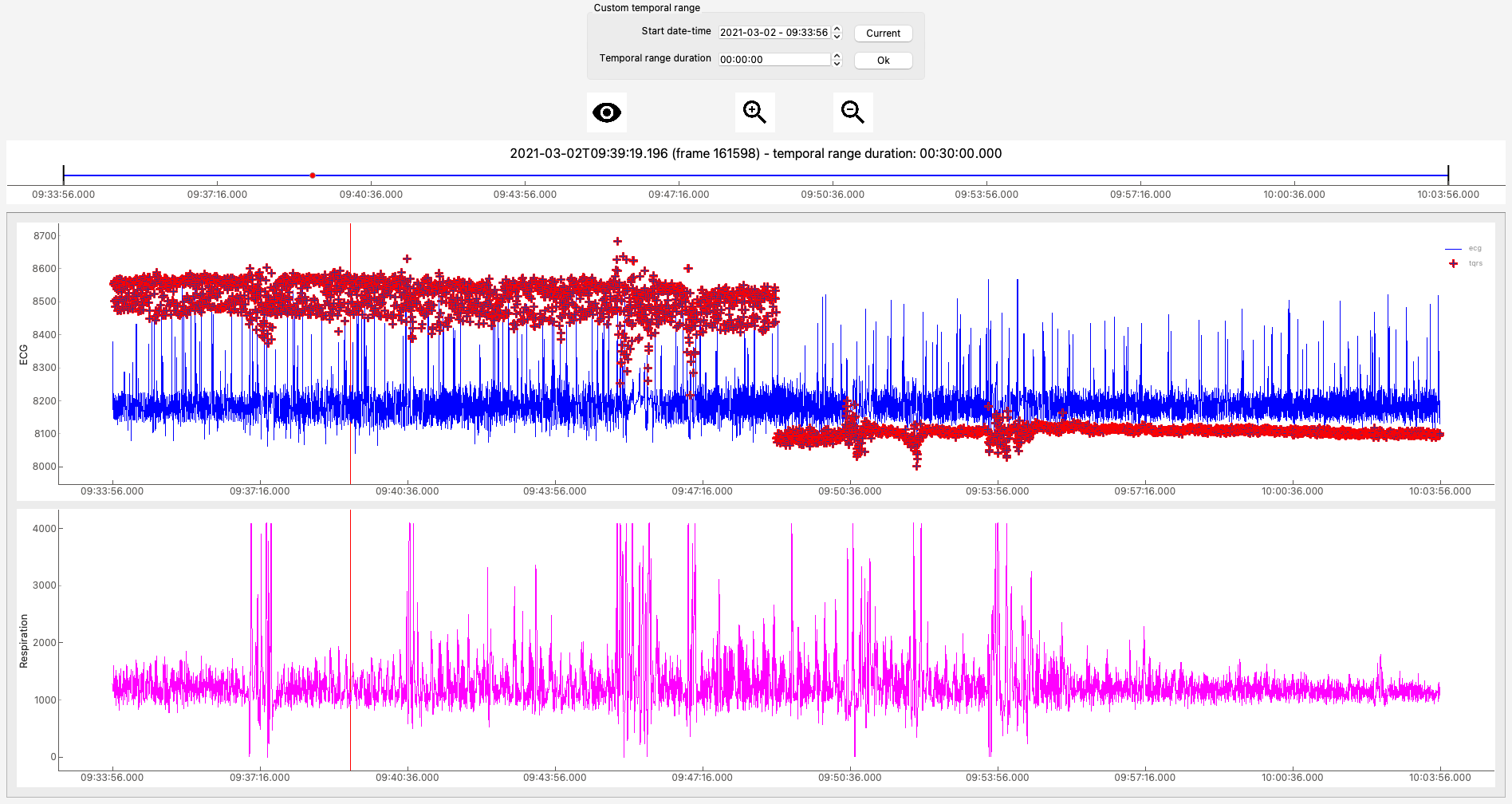
Fig. 3 Screenshot of ViSiAnnoT used as a signal viewer¶

Audio signal visualization¶

Regarding the visualization of an audio signal, the configuration is slightly different since the user must provide the channel to display (left or right). Here is an example:

from visiannot.visiannot import ViSiAnnoT

# audio path
path_audio = "data/Pat01_audio.wav"

# signal configuration
signal_dict = {}
signal_dict["Audio L"] = [[path_audio, '', None, '', "Left channel", 0, None]]
signal_dict["Audio R"] = [[path_audio, '', None, '', "Right channel", 0, None]]

# create ViSiAnnoT window
win_visiannot = ViSiAnnoT(
    {}, signal_dict, flag_pause_status=True, layout_mode=2
)

We define two signal widgets: “Audio L” and “Audio R”. They both take the same audio file as input.

In order to specify the channel to display in each plot, we use the key to access data and set it to “Left channel” and “Right channel”. The key word for channel selection is “left” or “right”, regardless of the letter capitalization and the position in the string. If no channel is specified, then the left channel is displayed by default.

The signal frequency is automatically retrieved from the wav file, so in the configuration list it can be set to anything (in this example 0).

The beginning datetime is not contained in the audio file name, so one of the three related variables is set to None and a default beginning datetime is defined (2000/01/01 00:00:00).

Fig. 4 shows a screenshot of the resulting window.

Fig. 4 Screenshot of ViSiAnnoT used as an audio signal viewer¶

Zoom tools¶

The default zoom of Pyqtgraph is available for the Y axis of the signal plots and is overwritten for the X axis so that all the signal widgets are linked. Thus the zoom tools described here only affects the temporal axis.

Based on Fig. 3, Fig. 5 illustrates the temporal zoom. We call “temporal range” the period of the signals that is displayed and “temporal range duration” its duration. In the progress bar, the black lines delimit the temporal range. We can see that the temporal range duration in Fig. 3 is 30min00s and becomes 00min36s after zoom in Fig. 5. The black lines of the progress bar have also moved to show what part of the signals is displayed.

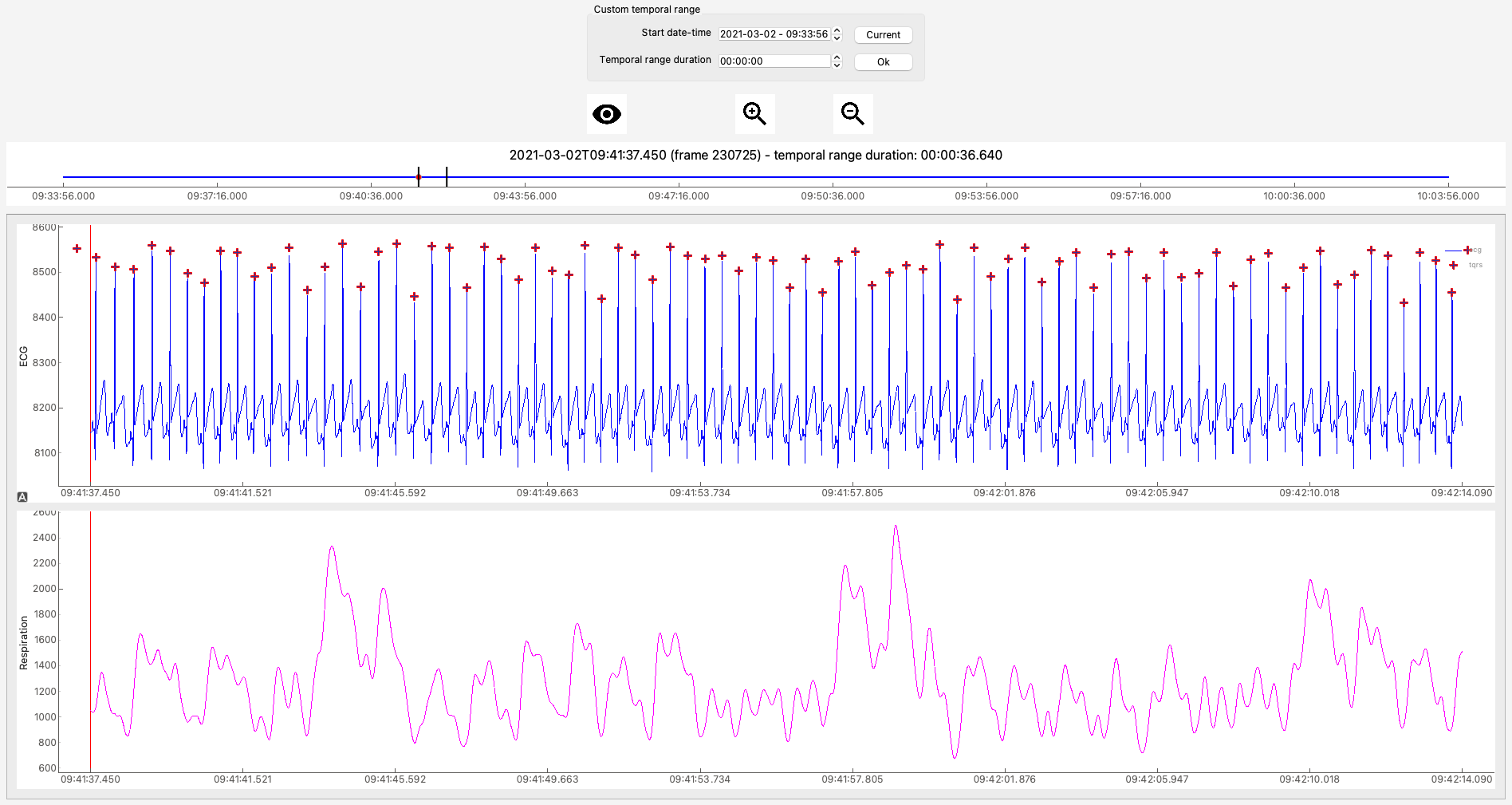
Fig. 5 Screenshot of ViSiAnnoT used as a signal viewer after zoom¶

The user can zoom in/out around the temporal cursor by using the two buttons looking like magnifying glass. It is also possible to directly zoom out in order to visualize the full signals by using the button looking like an eye. The buttons can be seen in the top left corner of the window.

YRange¶

The range of values on the Y axis of a specific signal widget may be fixed by the user.

This is done with the dictionary y_range_dict which is passed to ViSiAnnoT as a keyword argument. The key of the dictionary must correspond to a key of signal_dict, it specifies the signal widget where the Y range is fixed. The value of the dictionary is a tuple of length 2 with the minimum and maximum value on the Y axis.

Threshold values¶

Threshold values can be drawn as horizontal lines on a signal plot. It may be useful to identify temporal intervals where a signal is above or below a specific value.

This is done with the dictionary threshold_dict which is passed to ViSiAnnoT as a keyword argument. The key of the dictionary must correspond to a key of signal_dict, it specifies the signal widget where to draw the threshold. The value of the dictionary is a nested list of thresholds, each element is a list of length 2: threshold value and threshold color (RGB) or (RGBA).

Here is an example:

# threshold configuration
threshold_dict = {}
threshold_dict["RR"] = [
    [500, (51, 102, 0)],
    [600, (178, 34, 34)]
]

Fig. 6 shows an example of a signal widget with thresholds.

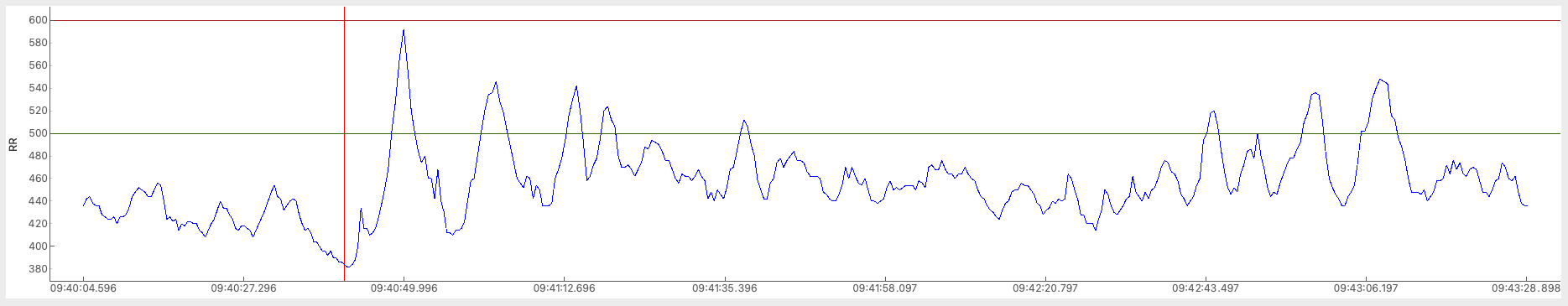
Fig. 6 Detail of a screenshot of ViSiAnnoT used as a signal viewer with two thresholds¶

Temporal intervals¶

It is also possible to display temporal intervals on the signal widgets. This may be useful if the user has pre-annotations or results from a detection algorithm and wants to visually check their accuracy.

This is done with the dictionary interval_dict which is passed to ViSiAnnoT as a keyword argument. The key of the dictionary must correspond to a key of signal_dict, it specifies the signal widget where to display temporal intervals. The value of the dictionary is a nested list of configurations for each kind of interval to display on the same widget. The configuration is a list of length 7:

Path to the interval file,
Delimiter to get the beginning datetime in the interval file name,
Position of the beginning datetime in the interval file name, according to the delimiter,
Format of the beginning datetime in the interval file name (see keyword argument fmt of convert_datetime_to_string()),
Key to access the data in the file (in case of .h5 or .mat, set it to '' otherwise),
Interval frequency (may also be a string with path to the frequency attribute in case of h5 file),
RGBA color.

The intervals may be stored in two ways in the files:

As a vector of length $n_{sample}$ with 0 and 1, where $n_{sample} \in \mathbb{N}$ is the number of samples in the file,
As a matrix of shape $(n_{inter},2)$ , where $n_{inter} \in \mathbb{N}$ is the number of intervals in the file, each line is an interval with the starting sample and the ending sample.

Here is an example:

from visiannot.visiannot import ViSiAnnoT

# signal paths
path_physio = "data/signal/Pat01_2021-03-02T09-33-56_physio.h5"
path_tqrs = "data/signal/Pat01_2021-03-02T09-33-56_tqrs.txt"
path_interval_a = "data/interval/Pat01_2021-03-02T09-33-56_intervalA.txt"
path_interval_b = "data/interval/Pat01_2021-03-02T09-33-56_intervalB.txt"

# define plot style
plot_style_tqrs = {
    'pen': None,
    'symbol': '+',
    'symbolPen': 'r',
    'symbolSize': 10
}

# signal configuration
signal_dict = {}
signal_dict["ECG"] = [
    [path_physio, '_', 1, "%Y-%m-%dT%H-%M-%S", "ecg", 500, None],
    [path_tqrs, '_', 1, "%Y-%m-%dT%H-%M-%S", "tqrs", 0, plot_style_tqrs]
]

# interval configuration
interval_dict = {}
interval_dict["ECG"] = [
    [path_interval_a, '_', 1, "%Y-%m-%dT%H-%M-%S", '', 500, (0, 255, 0, 50)],
    [path_interval_b, '_', 1, "%Y-%m-%dT%H-%M-%S", '', 500, (255, 200, 0, 50)]
]

# create ViSiAnnoT window
win_visiannot = ViSiAnnoT(
    {}, signal_dict, flag_pause_status=True, layout_mode=2,
    interval_dict=interval_dict
)

In this example, two kinds of intervals are defined on the "ECG" widget. A specific color is assigned to each kind of temporal intervals. Fig. 7 shows this particular plot.

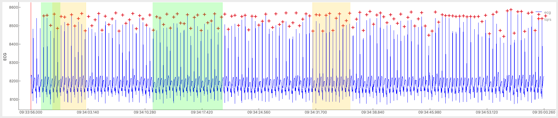
Fig. 7 Detail of a screenshot of ViSiAnnoT used as a signal viewer with additional temporal intervals¶

Combined video and signal visualization¶

ViSiAnnoT allows to combine video and signal visualization. The videos and the signals must be synchronized. If they do not share the same frequency, it is automatically taken into account.

Here is an example:

from visiannot.visiannot import ViSiAnnoT

# video paths
path_video_1 = "data/video/Pat01_2021-03-02T09-33-56_BW1.mp4"
path_video_2 = "data/video/Pat01_2021-03-02T09-33-56_BW2.mp4"

# video configuration
video_dict = {}
video_dict["BW1"] = [path_video_1, '_', 1, "%Y-%m-%dT%H-%M-%S"]
video_dict["BW2"] = [path_video_2, '_', 1, "%Y-%m-%dT%H-%M-%S"]

# signal paths
path_physio = "data/signal/Pat01_2021-03-02T09-33-56_physio.h5"
path_tqrs = "data/signal/Pat01_2021-03-02T09-33-56_tqrs.txt"

# define plot style
plot_style_tqrs = {
    'pen': None,
    'symbol': '+',
    'symbolPen': 'r',
    'symbolSize': 10
}

# signal configuration
signal_dict = {}

signal_dict["ECG"] = [
    [path_physio, '_', 1, "%Y-%m-%dT%H-%M-%S", "ecg", 500, None],
    [path_tqrs, '_', 1, "%Y-%m-%dT%H-%M-%S", "tqrs", 0, plot_style_tqrs]
]

# create ViSiAnnoT window
win_visiannot = ViSiAnnoT(video_dict, signal_dict)

Fig. 8 shows the resulting window. The temporal cursor is linked to the current video frame that is displayed. The user can navigate by clicking on a signal plot in order to change the position of the temporal cursor, then the video is displayed at the same position, as well as the navigation point in the progress bar. It is also possible to navigate by dragging the navigation point in the progress bar.

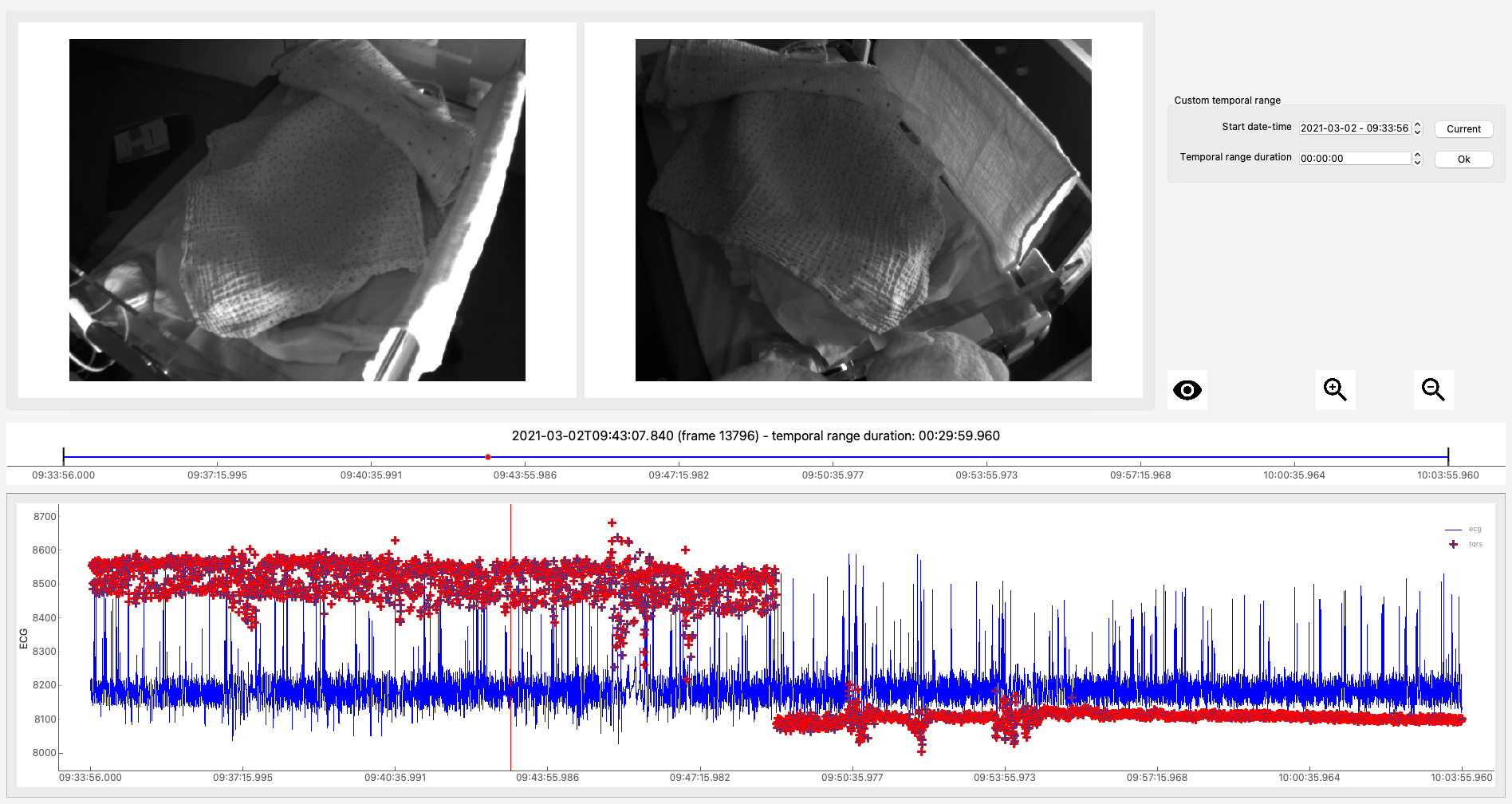
Fig. 8 Screenshot of ViSiAnnoT used as a combined video and signal visualizer¶

Tools for fast navigation¶

First, there is a combo box to select a temporal range duration in order to display a new temporal range that will begin at the current position of the temporal cursor. The list of available temporal range durations must be configured by the user with the keyword argument from_cursor_list in ViSiAnnoT constructor. For example, to have the choice between 30 seconds, 1 minute and 1 minute 30 seconds: from_cursor_list=[(0, 30), (1, 0), (1, 30)].

Second, there is a tool for defining a custom temporal range, as shown in Fig. 9. The user must define the start datetime of the temporal range. The push button “Current” can be used to define it as the current position of the temporal cursor. Then, the user must define the temporal range duration.

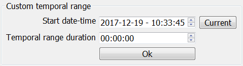
Fig. 9 Tool for defining a custom temporal range¶

Management of long recording¶

This section introduces the features for managing long recordings. All features introduced above are still available for long recordings. The class ViSiAnnoTLongRec inherits from ViSiAnnoT and adds specific features to manage long recordings.

A long recording is defined as a set of consecutive video and/or signal files. If we come back to the example dataset, we have a long recording composed of the following files:

Video
- Pat01_2021-03-02T09-33-56_BW1.mp4
- Pat01_2021-03-02T09-33-56_BW2.mp4
- Pat01_2021-03-02T10-03-56_BW1.mp4
- Pat01_2021-03-02T10-03-56_BW2.mp4
- Pat01_2021-03-02T10-33-56_BW1.mp4
- Pat01_2021-03-02T10-33-56_BW2.mp4
Signal
- physio_2021-03-02T09-34-09.h5

For both cameras, there are three consecutive video files of 30 minutes. The signals “ECG” and “Respiration” are both stored in one file which duration is 1h30min.

The long recording is divided into several consecutive even-time parts, also called “files”. The duration of the “files” is set with the keyword argument temporal_range of the constructor of ViSiAnnoTLongRec. It is a tuple of length 2 (minute, second). For the example dataset, temporal_range=(30, 0) would lead to a division of the recording into 3 “files”.

In the context of long recording, there are two additional buttons that allow to switch easily from one “file” to another and a combo box to directly select a specific “file” in the recording. Fig. 10 shows these buttons and the combo box.

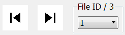
Fig. 10 Buttons and combo box for file selection in a long recording¶

We define the video configuration and the signal configuration almost the same way as for the class ViSiAnnoT, but instead of specifying the path to a file, we specify the directory containing the data files and a pattern to find them. We assume that the beginning datetime of each data file is contained in its name, which is required for synchronization.

Regarding video_dict, each item corresponds to one camera. The key is the camera ID and the value is a list of 5 elements:

Directory where to find the video files,
Pattern to find the video files,
Delimiter to get the beginning datetime in the video file name,
Position of the beginning datetime in the video file name, according to the delimiter,
Format of the beginning datetime in the video file name (see keyword argument fmt of convert_datetime_to_string()).

Regarding signal_dict, each item corresponds to one signal widget. The key is the widget ID. The value is a nested configuration list where each element corresponds to one signal to plot and is a list of 8 elements:

Directory where to find the signal files,
Pattern to find the signal files,
Delimiter to get the beginning datetime in the signal file name,
Position of the beginning datetime in the signal file name, according to the delimiter,
Format of the beginning datetime in the signal file name (see keyword argument fmt of convert_datetime_to_string()),
Key to access the data in the file (in case of .h5 or .mat, set it to '' otherwise), also used a legend - in case of 2D data with several value columns, then the column index must be specified, e.g. "key - 1" or "key - colName" if there is an attribute at key named columns with columns name being comma-separated (first column is always the timestamps),
Signal frequency (may also be a string with path to the frequency attribute in case of h5 file), set it to 0 in case of non-regularly sampled signal,
Dictionary with plot style.

Here is an example:

from visiannot.visiannot import ViSiAnnoTLongRec

# data directory
dir_vid = "data/video"
dir_sig = "data"

# video configuration
video_dict = {}
video_dict["BW1"] = [dir_vid, "*BW1*.mp4", '_', 1, "%Y-%m-%dT%H-%M-%S"]
video_dict["BW2"] = [dir_vid, "*BW2*.mp4", '_', 1, "%Y-%m-%dT%H-%M-%S"]

# signal configuration
signal_dict = {}
signal_dict["ECG"] = [[dir_sig, "physio_*.h5", '_', 1, "%Y-%m-%dT%H-%M-%S", "ecg", 500, None]]
signal_dict["Respiration"] = [[dir_sig, "physio_*.h5", '_', 1, "%Y-%m-%dT%H-%M-%S", "resp", "resp/freq", None]]

# create ViSiAnnoT window
win_visiannot = ViSiAnnoTLongRec(
    video_dict, signal_dict, flag_pause_status=True, temporal_range=(30, 0)
)

Synchronization of the different modalities¶

Let’s give an example of synchronization of a long recording with three modalities. Below we give the timestamp and duration of the data files.

Video: 3 files
- 2000/01/01, 00h00m20s - 45 seconds
- 2000/01/01, 00h01m05s - 25 seconds
- 2000/01/01, 00h01m50s - 45 seconds
Signal regularly sampled (signal 1D): 3 files
- 2000/01/01, 00h00m35s - 30 seconds
- 2000/01/01, 00h01m30s - 50 seconds
- 2000/01/01, 00h02m20s - 30 seconds
Signal not regularly sampled (signal 2D): 3 files
- 2000/01/01, 00h00m00s - 50 seconds
- 2000/01/01, 00h01m05s - 45 seconds
- 2000/01/01, 00h01m50s - 45 seconds

We choose a temporal range of 60 seconds for dividing the long recording into several “files”, see Example of synchronization.

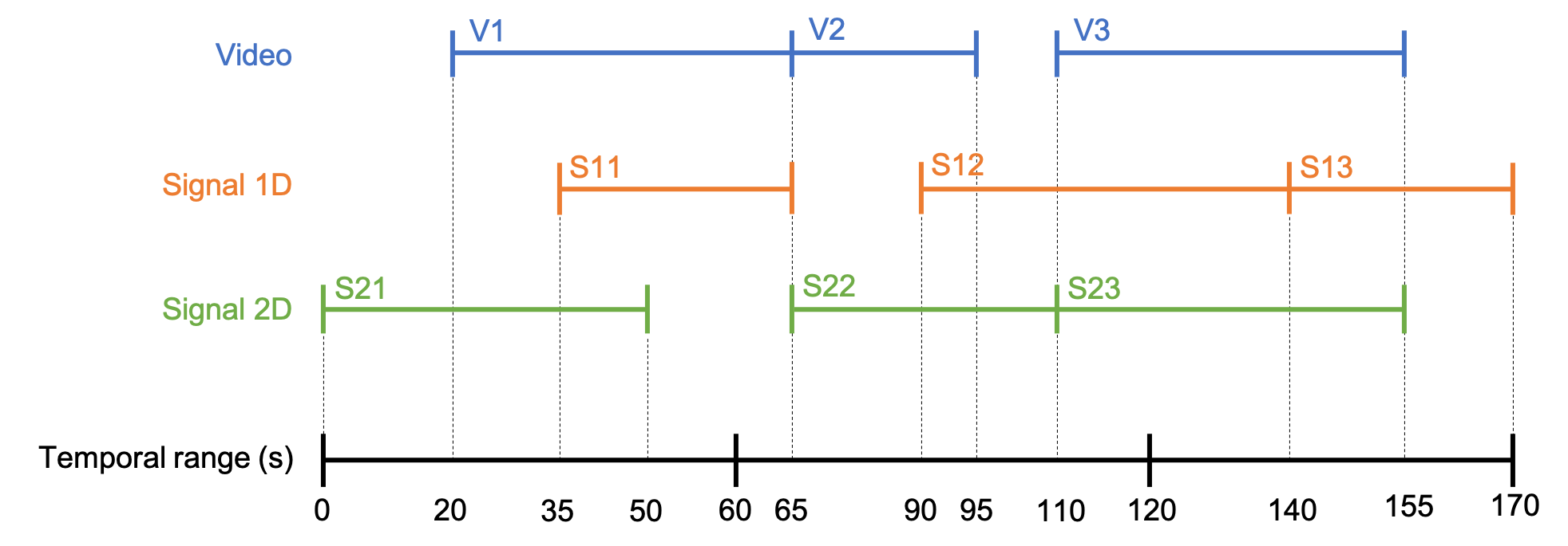
Fig. 11 Example of synchronization¶

In order to synchronize the different modalities with each other, ViSiAnnoTLongRec first creates a set of temporary synchronization files with the method process_synchronization_all(), stored in the folder sig-tmp. For each modality, a temporary file is created for each “file” of the long recording. The temporary file give all necessary information to get data spanning the corresponding “file” in the long recording.

The set of temporary files begin at the earliest timestamp of all data files of all modalities (in the example, at 2000/01/01, 00h00m00s). The last “file” of the long recording is truncated if necessary so that it ends at the last sample of all data files of all modalities (in the example, instead of lasting 60 seconds, it lasts 50 seconds). In the example, there are 3 “files” in the long recording.

The content of the temporary files depends on the data type (video, signal 1D or signal 2D). Basically, they contain the list of data files spanning the corresponding “file” in the long recording and the temporal offset relatively to the beginning of the corresponding “file”.

For video, here is the content of the temporary synchronization files:

File at 00h00m00s      File at 00h01m00s      File at 00h02m00s
V1 *=* 20 *=* 60       V1 *=* -40 *=* 5       V3 *=* -10 *=* 155
                       V2 *=* 5 *=* 30
                       V3 *=* 50 *=* 60

Each line contains the path to the video file, its beginning and ending timestamp in the “file” of the long recording. A negative beginning timestamp means that the video file begins before the “file” in the long recording.

For signal 1D, here is the content of the temporary synchronization files:

File at 00h00m00s      File at 00h01m00s      File at 00h02m00s
None *=* 35            S11 *=* -25            S12 *=* -30
S11                    None *=* 25            S13
                       S12

If the path to signal file is None, then it means that there is no data during the associated number of seconds. If the associated number of seconds is negative, then it means that the signal file begins before the “file” in the long recording. Otherwise, the whole signal file is used.

For signal 2D, here is the content of the temporary synchronization files:

File at 00h00m00s      File at 00h01m00s      File at 00h02m00s
S21 *=* 0              S22 *=* 5              S23 *=* -10
                       S23 *=* 50

Each line contains the path to the signal file and its beginning timestamp in the “file” of the long recording. A negative beginning timestamp means that the signal file begins before the “file” in the long recording.

The method get_synchro_signal() is used to read the temporary synchronization file and gets the signal array that is synchronized with the current “file” in the long recording.

Multi-label annotation tools¶

ViSiAnnoT provides two annotation tools:

Temporal events annotation,
Image extraction.

Events annotation tool¶

This tool allows to annotate temporal intervals. The user can provide as much labels as desired. This tool is useful for establishing the ground truth of a temporal segmentation or classification, as well as studying the occurrence and duration of specific events. It automatically creates a file for each label, where the annotations are written.

When creating an instance of ViSiAnnoT or ViSiAnnoTLongRec, the configuration dictionary of the annotation tool is given to the keyword argument annotevent_dict of the constructor. Here is an example:

annotevent_dict = {}
annotevent_dict["Label-1"] = [200, 105, 0, 50]
annotevent_dict["Label-2"] = [105, 205, 0, 50]

There are two labels (dictionary keys), to which is associated a color (dictionary values).

Fig. 12 shows a screenshot of the events annotation tool.

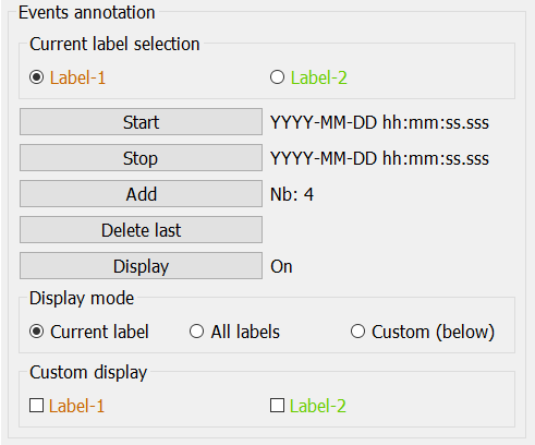
Fig. 12 Events annotation tool¶

The radio buttons on the top allow to select the current label. The push buttons “Start” and “Stop” respectively set the beginning and ending datetime of the annotated temporal interval. In this example, the ending datetime is not defined yet. The push button “Add” validates the annotation and appends it in a file. The number of annotations is displayed next to it. The push button “Delete last” deletes the last added annotation. The push button “Display” enables or disables the display of the annotations on the signals plots.

The “Display mode” radio buttons allow to choose what to display:

“Current label”: only the annotations of the current label is displayed (current label is the one selected in the “Current label selection” box),
“All labels”: the annotations of all labels are displayed,
“Custom (below)”: the user can choose the labels to display thanks to the check boxes below.

Fig. 13 shows a screenshot of two signal plots with annotations displayed. They are displayed similarly to the additional temporal intervals. Each color corresponds to one label. As it can be seen on the progress bar, the temporal range is the first 5 minutes. The annotations outside of the temporal range are still displayed on the progress bar.

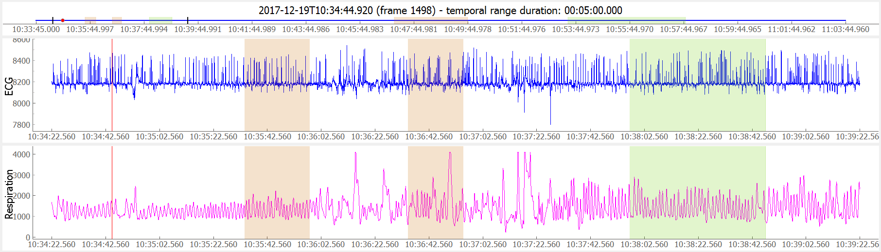
Fig. 13 Detail of a screenshot of ViSiAnnoT with annotations displayed, each color corresponding to one label¶

It is possible to display the duration of the annotated intervals by clicking with the left button of the mouse while pressing the alt key. The label of the annotated interval must be the current label in order to get the display. An example is given in Fig. 14.

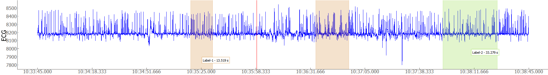
_images/annotation_event_description.png

Fig. 14 Detail of a screenshot of ViSiAnnoT with annotations displayed, two of them with duration displayed¶

By default, it is not possible to overlap two annotations with the same label. In order to enable this feature, the keyword argument flag_annot_overlap of ViSiAnnoT constructor must be set to True.

Storage of events annotation¶

In the constructor of ViSiAnnoT, the keyword argument annot_dir specifies the directory where to store annotation files. By default it is the directory “Annotations”, located at the current working directory from where ViSiAnnoT is launched.

For each label, a text file is created with the intervals of the annotated events. The name of the annotation file is BASENAME_LABEL, where BASENAME is the basename of the annotation directory and LABEL is the label.

Each line in an annotation file corresponds to an annotated event: TS1 - TS2, where TS1 (resp. TS2) is the start (resp. stop) timestamp of the annotated event. The timestamp is formatted as follows: %Y-%m-%dT%H:%M:%S.%f, where %Y is the year in 4 digits, %m is the month in 2 digits, %d is the day in 2 digits, %H is the hour, %M is the minute, %S is the second and %f is the microsecond.

Image extraction tool¶

This tool allows to extract a still image from the video(s) and associate a label to it.

When creating an instance of ViSiAnnoT or ViSiAnnoTLongRec, the configuration of the annotation tool is given to the keyword argument annotimage_list. Here is an example:

annotimage_list = ["Label-A", "Label-B", "Label-C"]

Fig. 15 shows a screenshot of the image extraction tool. The user selects the label thanks to the radio buttons. Then the push button “Save” allows to extract the current frame for each camera and saves it in a directory named after the selected label.

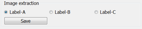
Fig. 15 Image extraction tool¶

The extracted images are stored in the same directory than events annotation files. For each label, a sub-directory is created, named after the label, where are stored the extracted images. The image file name is "%s_%d.png", where %s is the video file name and %d is the frame index of the image.

Layout modes¶

In the context of combined video and signal visualization, the user may want to put the emphasis on either the video or the signal. For this purpose, we provide four default layout mode, to be selected with the keyword argument layout_mode (may be 1, 2, 3 or 4). The user may also manually configure the layout of the window with the keyword argument poswid_dict.

Here is an example of combined video and signal visualization in the context of long recording with all features enabled (events annotation, image extraction, tools for fast navigation):

from visiannot.visiannot import ViSiAnnoTLongRec

# data directory
dir_vid = "data/video"
dir_sig = "data"

# video configuration
video_dict = {}
video_dict["BW1"] = [dir_vid, "*BW1*.mp4", '_', 1, "%Y-%m-%dT%H-%M-%S"]
video_dict["BW2"] = [dir_vid, "*BW2*.mp4", '_', 1, "%Y-%m-%dT%H-%M-%S"]

# define plot style
plot_style_tqrs = {
    'pen': None,
    'symbol': '+',
    'symbolPen': 'r',
    'symbolSize': 10
}

# signal configuration
signal_dict = {}
signal_dict["ECG"] = [
    [dir_sig, "physio_*.h5", '_', 1, "%Y-%m-%dT%H-%M-%S", "ecg", 500, None],
    [dir_sig, "physio_*.h5", '_', 1, "%Y-%m-%dT%H-%M-%S", "beat - TQRS", 0, plot_style_tqrs]
]
signal_dict["RR"] = [[dir_sig, "physio_*.h5", '_', 1, "%Y-%m-%dT%H-%M-%S", "beat - RR", 0, None]]

# event annotation dictionary
annotevent_dict = {}
annotevent_dict["Label-1"] = [200, 105, 0, 50]
annotevent_dict["Label-2"] = [105, 205, 0, 50]

# image annotation dictionary
annotimage_list = ["Label-A", "Label-B"]

# create ViSiAnnoT window
win_visiannot = ViSiAnnoTLongRec(
    video_dict, signal_dict,
    flag_pause_status=True,
    temporal_range=(5, 0),
    annotevent_dict=annotevent_dict,
    annotimage_list=annotimage_list,
    from_cursor_list=[(0, 30), (1, 0), (2, 0)],
    layout_mode=1
)

Mode 1 puts the emphasis on the video. If there is not enough space left for the signals, a scroll area is created.

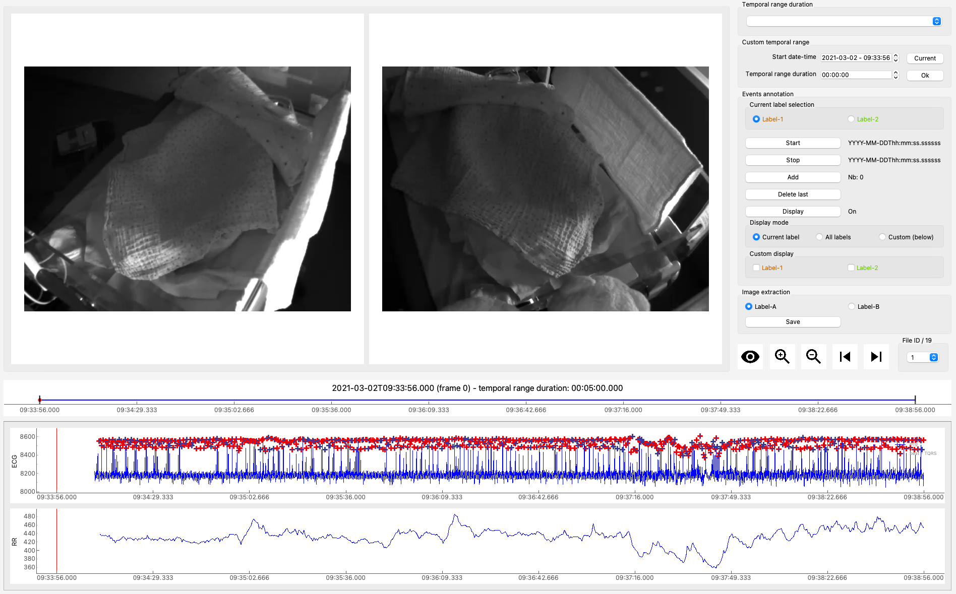
Fig. 16 Layout mode 1¶

Mode 2 puts the emphasis on the signal.

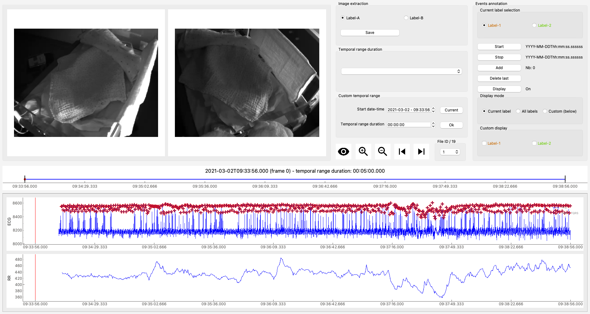
Fig. 17 Layout mode 2¶

Mode 3 provides a more compact display since the following features are disabled: selection of temporal range from cursor, and custom selection of temporal range.

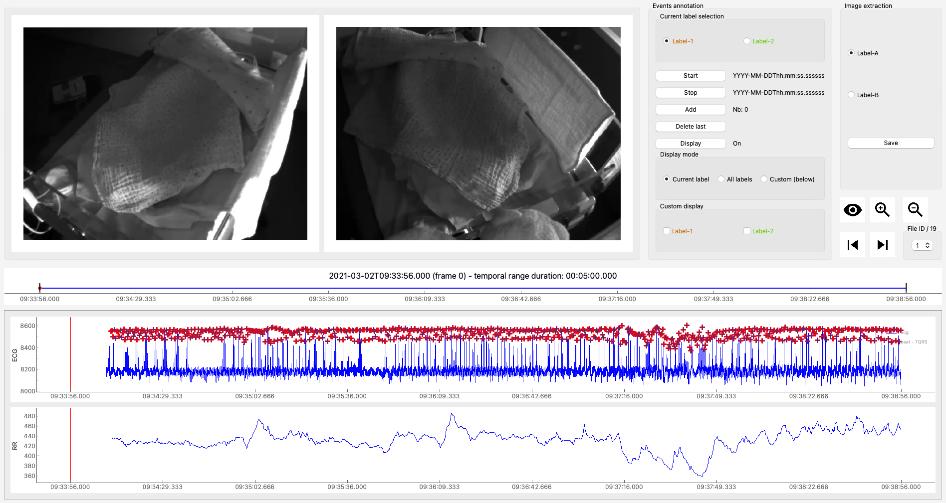
Fig. 18 Layout mode 3¶

Mode 4 is adapted to portrait screen orientation.

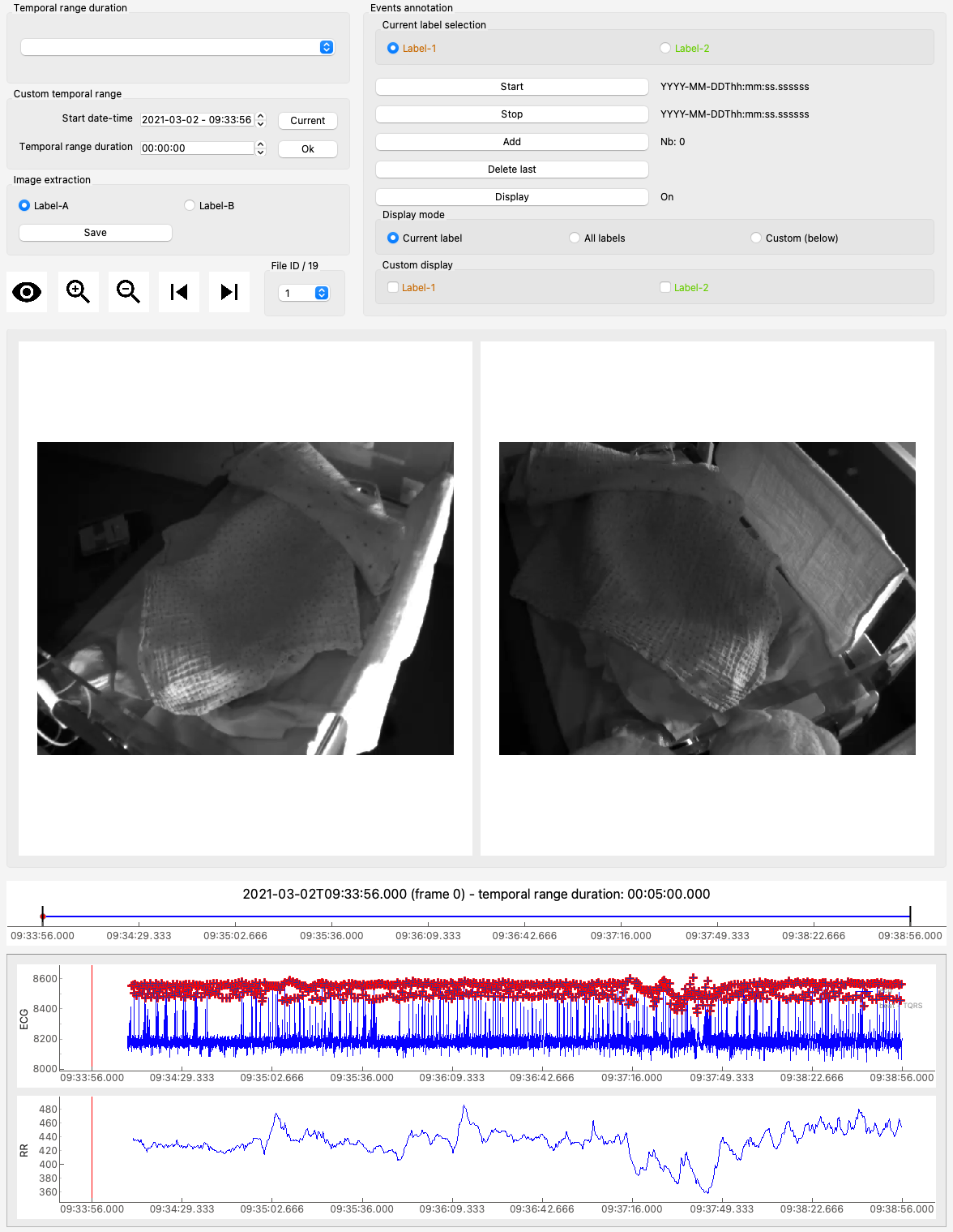
Fig. 19 Layout mode 4¶

Keyboard/mouse interactions¶

Here is a synthesis of all the possible user interactions with the keyboard and the mouse.

Keyboard¶

Press

space: start/stop of the video playback
left: 1 second backward
- with control pressed: 1 minute backward
right: 1 second forward
- with control pressed: 1 minute forward
down: 10 seconds backward
- with control pressed: 10 minutes backward
up: 10 seconds backward
- with control pressed: 10 minutes backward
l: 1 sample backward
m: 1 sample forward
i: zoom in
o: zoom out
n: whole zoom out
a: start annotation
z: stop annotation
e: add annotation
s: display annotations
page down: switch to previous file (in long recordings only)
page up: switch to next file (in long recordings only)
home: set the position of the temporal cursor to the first sample of the current file
end: set the position of the temporal cursor to the last sample of the current file
d + control + shift: delete the display of annotation durations

Release

alt: show/hide the menu bar

Mouse click on the signal plots¶

left button: define the new position of the temporal cursor
- with both control and shift pressed: delete the annotation that is clicked on (the label must be the current label)
- with alt pressed: enable or disable to display the duration of the annotation that is clicked on (the label must be the current label)
right button: zoom in (3 clicks: the first two to define the new temporal range, the third click must be inside the new temporal range in order to validate and zoom in, or outside to cancel)
- with control pressed: add events annotation (3 clicks: the first two to define the start/stop of the annotation, the third click must be inside the temporal range in order to add the annotation, or outside to cancel)